 www.pi314.net |
|
The world of Pi - V2.57 modif. 13/04/2013 |
|
|
|
|
|
|
![]()
![]()

Fast Multiplication by FFT
1 Back
to school
If you were asked to multiply 32*14 in your head, how would you go
about it? Most likely, while painfully rembering those every long rules
taught in primary school, use 32=3*10+2, 14=10+4, then multiply
each part with each part, remembering any caries over etc. Phew, it
seems to be the easiest way... But is it really? This sounds like a
weird question, no?
Since the comming a calculators, that is since
the late 40s, the gap of useful algorithm for multiplication force us
to break each number into smaller parts, for example at school  .
Hence the multiplicaiton of size
.
Hence the multiplicaiton of size  needed then a time (or number of operations)
proportional to
needed then a time (or number of operations)
proportional to  without taking into account the usage of a memory
storage proportional to
without taking into account the usage of a memory
storage proportional to  .
So to conserve the progression speed of the record of decimals of
calculated during the 50s
(see History or Decimals page), some theoretical and
algorithmical improvement were in great need. So it was during this
period that things speeded up.
.
So to conserve the progression speed of the record of decimals of
calculated during the 50s
(see History or Decimals page), some theoretical and
algorithmical improvement were in great need. So it was during this
period that things speeded up.
In 1965, Cooley and Tukey introduced in it's
modern form a method to reduce the complexity of calculating Fourier's
serie, that is now known as Fast Fourier Transform (FFT) [1]. It seems
that Gauss had already guessed the trick of
critical factorisation in 1805. No doubt, he was a pure genius...
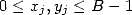
Anyway, Schönhage and Strassen produced an algorithm to multiply
to big integers with complexity  which is considerably
much better than
which is considerably
much better than  [2]
!
[2]
!
This page explain how this algorithm for fast
multiplication of two big integers by FFT works, which did so much for
the calculation of the decimals of  ! For the computers, this is great... But for us, well,
hum... actually our brain are not wired to function in that way !
! For the computers, this is great... But for us, well,
hum... actually our brain are not wired to function in that way !
2 Algorithm for fast multiplication of two large integers by FFT
Let X and Y be two large integers of size  in base
  (or of power
  ).
).
2.1 Polynomial decomposition
We write  and
and  in polynomial form by decomposing them (in a unique way)
in base
in polynomial form by decomposing them (in a unique way)
in base 
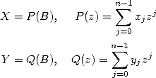
where  and
and  are therefore respectively the
  th decimales of
  and
and  (
( ). This calculation is
roughly of complexity proportional to
). This calculation is
roughly of complexity proportional to  . We now look how to "quickly" calculate the
multiplication
. We now look how to "quickly" calculate the
multiplication 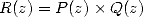 then in the end evaluate
  .
.  is a polynomial of degree
  and can be found by interpolation by evaluating it in
  points, in other words by evaluating
  and
and  in those same
  points. Choosing those points, is the magical trick of
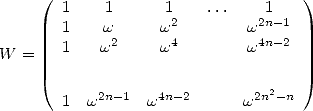
this algorithm! We use the
points. Choosing those points, is the magical trick of
this algorithm! We use the  th root of unity, i.e.
 |
(3) |
since this evaluation (which is none the other
than the calculation of a Fourier's serie) can be done in complexity  if
if  is a power of
  and with a bit of cleverness. This is Fast Fourier
Transform or FFT.
and with a bit of cleverness. This is Fast Fourier
Transform or FFT.
2.2 Fast
Fourier Transform
By keeping the previous notation, let's
evaluate the polynomials  and
and  with the hypothesis that
  . Then
and  . So we get
 |
(6) |
Now, we remember that since  is a
is a  th root of unity, then for
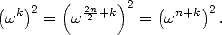 |
(7) |
From this, evaluating  to the
  th root of unity come down to evaluating both
  and
and  at the
  points
 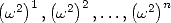 and
put the result back in
and
put the result back in  with the help of equation 6.
If
with the help of equation 6.
If  is the number of elementary opreations
(addition,
multiplication) needed to evaluate
is the number of elementary opreations
(addition,
multiplication) needed to evaluate  in
in 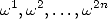 then in accordance to the previous
principle and of 6,
we get
then in accordance to the previous
principle and of 6,
we get
 |
(8) |
where the term  comes from the last additions and multiplications needed
to obtain
comes from the last additions and multiplications needed
to obtain  from
from  and
and  in 6.
in 6.
Since  is a
is a  th root of unity, we can reapply the same process for
each polynomial
th root of unity, we can reapply the same process for
each polynomial  and
and  . It follows that, since
  is a power of
  , the process (and hence 6)
is iterated an other
, the process (and hence 6)
is iterated an other  times. We finnaly get a number of operations
 |
(9) |
where the complexity is  of FFT. Similarly for the inverse FFT
, which uses
of FFT. Similarly for the inverse FFT
, which uses  instead of
  .
.
2.3 Interpolation
We have now worked out our  and
and  for
for  . We create the
  products
  whcih
comes back to elementary multiplication since
whcih
comes back to elementary multiplication since  has obviously modulo less than
  using 1, similarly for
  . Since we are looking to find
  , we need to interpolate
from the
, we need to interpolate
from the  values
  . In other words we are
looking to solve the system
. In other words we are
looking to solve the system
 |
(10) |
where
 |
(11) |
which is equivalent to
 |
(12) |
where  has the great idea of being simply
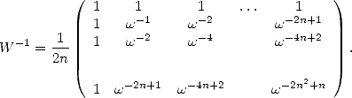 |
(13) |
Calculating 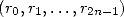 is no other than the conjugate
of Fourier Transform's of
is no other than the conjugate
of Fourier Transform's of 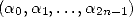 , in other words it's inverse
Fourier Transform, so we saw that it is in
, in other words it's inverse
Fourier Transform, so we saw that it is in  like FFT. We then get
  where we can find
  . This last operation is roughly of complexity
  since the
  are already close to the
decimals of
are already close to the
decimals of  , plus or minus the carry overs (as soon as
  ). All the carry overs are simultaneously calculated, then carried
through, then we recalculate any new carry over created, etc.... (an
operation called vectorizing).
). All the carry overs are simultaneously calculated, then carried
through, then we recalculate any new carry over created, etc.... (an
operation called vectorizing).
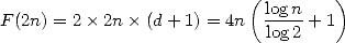
The combination of all those algorithm and a
few small refining done by programmers allow us to reach roughly the
theoretical optimal barrier of Schönhage and Strassen for the FFT
in  .
.
References
[1] J. W. Cooley, J. W. Tukey, “An algorithm for the machine calculation of complex Fourier series”, Math. Comp. 1965, vol 19, pp. 297-301.
[2] A. Schönhage, V. Strassen, “Schennelle Multiplikation grosser Zahlen”, Computing, 1971, vol. 7, pp. 281-292.
back to home page